Tag Archives: quantile regression

Outliers in Analysis

This is a post I wrote on company's internal wiki... just want a backup here.

Three points to bear in mind:

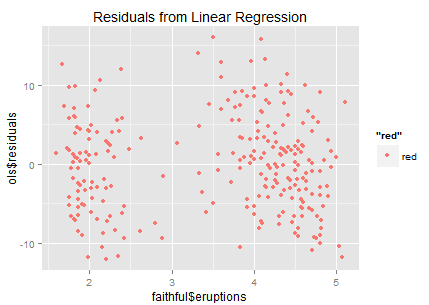
  1. Outliers are not bad; they just behave differently.
  2. Many statistics are sensitive to outliers. e.g. the mean and every model that relies on the mean.
  3. Abnormal detection is another topic; this post focus on exploring robust models.

Make the analysis robust to outliers:

Method
Action
Advantage
Concern
Remove the outliers remove outliers according to a certain threshold or calculation (perhaps via unsupervised models); only focus on the left subsample. In most cases the signal will be more clear from concentrated subsample. Hard to generalize the effect to entire population; hard to define a threshold.
Capping the outliers cap the outliers to a certain value. All observations are kept so easy to map the effect to all samples afterward; outliers' impacts are punished. softer compared to removing the outliers; hard to find the threshold or capping rule.
Control for covariates include some control variables in the regression. some how analyze the "difference" but not just linear and constant difference. Introduce some relevant factors to gain a precise estimation and better learning. Need to find the right control variable. Irrelevant covariates will only introduce noise.
Regression to the median Median is more robust than the mean when outliers persist. Run a full quantile regression if possible; or just 50% quantile which is the median regression. Get a clear directional signal; robust to outliers so no need to choose any threshold. Hard to generalize the treatment effect to all population.
Quantile Regression Generalized model from above; help you understand subtle difference in each quantile. Gain more knowledge on the distribution rather than single point and great explanation power. Computational expensive; hard for further generalization;
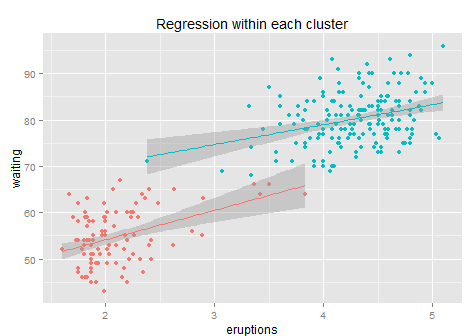
Subsample Regression Instead of regress to each quantile, a subsample regression only run regression within each strata of the whole sample (say, sub-regression in each decile). Identical to introducing a categorical variable for each decile in regression; also help inspect each subsample. only directional; higher accumulated false-positive rate.
Take log() or other numerical transformations It's a numerical trick that shrink the range to a narrower one (high punishment on the high values). Easy to compute and map back to the real value; get directional results. May not be enough to obtain a clear signal.
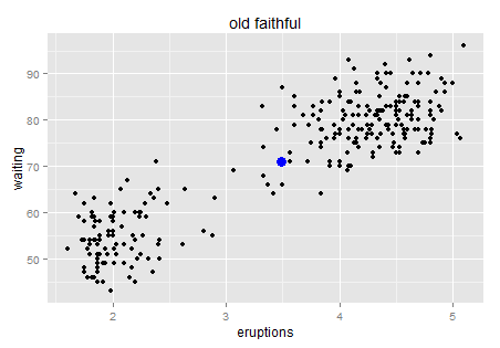
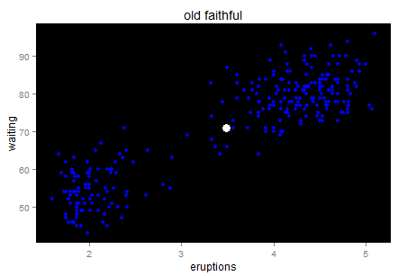
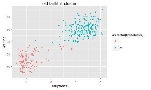
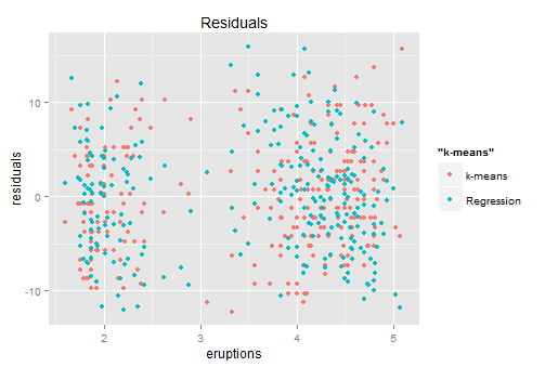
Unsupervised study for higher dimensions This is more about outlier detection. When there are more than one dimension to define an outlier, some unsupervised models like K-means would help (identify the distance to the center). deals with higher dimensions exploration only.


Rank based methods Measure ranks of outcome variables instead of the absolute value. immunized to outliers. Hard to generalize the treatment effect to all population.


That's all I could think of for now...any addition is welcome 🙂

------- update on Apr 8, 2016 --------

Some new notes:

  1. "outliers" may not be the right name for heavy tails.
  2. Rank methods.

Variance: regression, clustering, residual and variance

This is the translation of my recent post in Chinese. I was trying to talk in the way that a statistician would use after having stayed along with so many statistics people in the past years.

-------------------------------------------Start----------------------------

Variance is an interesting word. When we use it in statistics, it is defined as the "deviation from the center", which corresponds to the formula  , or in the matrix form (1 is a column vector with N*1 ones). From its definition it is the second (order) central moment, i.e. sum of the squared distance to the central. It measures how much the distribution deviates from its center -- the larger the sparser; the smaller the denser. This is how it works in the 1-dimension world. Many of you should be familiar with these.

Variance has a close relative called standard deviation, which is essentially the square root of variance, denoted by . There is also something called the six-sigma theory-- which comes from the 6-sigma coverage of a normal distribution.

79f0f736afc37931c22b82ecebc4b74542a911b7.jpg

Okay, enough on the single dimension case. Let's look at two dimensions then. Usually we can visualize the two dimension world with a scatter plot. Here is a famous one -- old faithful.

2014-12-27 23_41_46-Plot ZoomOld faithful is a "cone geyser located in Wyoming, in Yellowstone National Park in the United States (wiki)...It is one of the most predictable geographical features on Earth, erupting almost every 91 minutes." We can see there are about two hundreds points in this plot. It is a very interesting graph that can tell you much about Variance.

Here is the intuition. Try to use natural language (rather than statistical or mathematical tones) to describe this chart, for example when you take your 6 year old kid to the Yellowstone and he is waiting for next eruption. What would you tell him if you have this data set? Perhaps "I bet the longer you wait, the longer next eruption lasts. Let's  count the time!". Then the kid has a glance on your chart and say "No. It tells us that if we wait for more than one hour (70 minutes) then we will see a longer eruption in the next (4-5 minutes)". Which way is more accurate?

Okay... stop playing with kids. We now consider the scientific way. Frankly, which model will give us a smaller variance after processing?

Well, always Regression first. Such a strong positive relationship, right?  ( no causality.... just correlation)

2014-12-27 23_51_53-Plot Zoom

Now we obtain a significantly positive line though R-square from the linear model is only 81% (could it be better fitted?). Let's look at the residuals.

2014-12-27 23_59_10-Plot ZoomIt looks like that the residuals are sparsely distributed...(the ideal residual is white noise which carries no information). In this residual chart we can roughly identify two clusters -- so why don't we try clustering?

Before running any program, let's have a quick review the foundations of the K-means algorithm. In a 2-D world, we define the center as , then the 2-D variance is the sum of squares of each pint going to the center.

2014-12-28 00_09_03-Plot ZoomThe blue point is the center. No need to worry about the outlier's impact on the mean too much...it looks good for now. Wait... doesn't it feel like the starry sky at night? Just a quick trick and I promise I will go back to the key point.


2014-12-28 00_25_06-Plot Zoom

For a linear regression model, we look at the sum of squared residuals - the smaller the better fit is. For clustering methods, we can still look at such measurement: sum of squared distance to the center within each cluster. K-means is calculated by numerical iterations and its goal is to minimize such second central moment (refer to its loss function). We can try to cluster these stars to two galaxies here.

2014-12-28 00_32_00-Plot ZoomAfter clustering, we can calculate the residuals similarly - distance to the central (represents each cluster's position). Then the residual point.


2014-12-28 00_51_13-Plot ZoomRed ones are from K-means which the blue ones come from the previous regression. Looks similar right?... so back to the conversation with the kid -- both of you are right with about 80% accuracy.

Shall we do the regression again for each cluster?

2014-12-28 01_01_20-Plot ZoomNot many improvements. After clustering + regression the R-square increases to 84% (+3 points). This is because within each cluster it is hard to find any linear pattern of the residuals, and the regression line's slope drops from 10 to 6 and 4  respectively, while each sub-regression only delivers an R-square less than 10%... so not much information after clustering.  Anyway, it is better than a simple regression for sure. (the reason why we use k-means rather than some simple rules like x>3.5 is that k-means gives the optimized clustering results based on its loss function).

Here is another question: why do not we cluster to 3 or 5? It's more about overfitting... only 200 points here. If the sample size is big then we can try more clusters.

Fair enough. Of course statisticians won't be satisfied with these findings. The residual chart indicates an important information that the distribution of the residuals is not a standard normal distribution (not white noise). They call it heteroscedasticity. There are many forms of heteroscedasticity. The simplest one is residual increases when x increases. Other cases are in the following figure.

p109figureThe existence of heteroscedasticity makes our model (which is based on the training data set) less efficient. I'd like to say that statistical modelling is the process that we fight with residuals' distribution -- if we can diagnose any pattern then there is a way to improve the model. The econometricians prefer to name the residuals "rubbish bin" -- however it is also a gold mine in some sense. Data is a limited resource... wasting is luxurious.

Some additional notes...

Continue reading